Here is the first article of a series, concerning the modelling and evaluation of the effect of seeing on telescopes of different diameters and characteristics.
This post follows a discussion on Cloudy Nights forum and another on a Italian forum. The discussions have been useful to better point out possible pitfalls, misunderstandings, and critical aspects of the modelling.
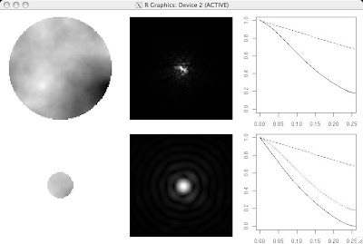
The picture shows the comparison of the Point Spread Function (a star image in focus) and of the MTFs for two unobstructed apertures in bad seeing conditions. Full aperture is on the first row, and aperture masked down to 1/4 diameter, is the second row,
The first thing that must be clearly understood is how the turbulent wavefront was generated for both cases. First I used the Suiter's model (which I have checked to produce turbulence intensities, at different wavelengths, which agree with the Kolmogorov's seeing model - I will return on this point). I calculated a random wavefront for the full aperture with a value of 0.3 waves rms. This is a large amount of turbulence, roughly corresponding to Fried's radius r0 equal to 1/4 the diameter. The generated wavefront is shown at top left of the picture (for one run, but since turbulence is generated by a random process one my get different results every time).
The wavefront for the 1/4 aperture is shown at bottom left. It is the same wavefront above but limited to the part seen by the 1/4 diameter. As can be seen the wavefront on the central part leaves out most of the fluctuations than happens on the full aperture. What remain is mostly a tilted wavefront. The overall amount of turbulence, excluding tilt is a lot less (it follows the Kolmogorov's prediction which say the rms value is proportional to (D/r0)^(5/6)).
The top centre picture is the star's image produced by the wavefront at top left. Since the diameter of the aperture is about (more than) 4 times the radius of the turbulence we can see a speckle structure with a number of speckles of about (more than) 16 false airy spots. Each spot is the size of the airy disk of the full aperture, but they are spread over an area the size of an hypothetical scope of diameter r0 (~4 times larger).
The bottom centre figure is the star's image corresponding to the wavefront of the reduced aperture (bottom left). In this case Fried's parameter r0 is about the same size of the masked aperture. In this case the airy disk is only minimally affected. There is only one, deformed airy disk, and the rings are irregular (actually r0 is slightly smaller than D/4 in this example).
The pictures are shown to the same scale. As can be seen the overall speckle size is about the same size than the disk of the masked aperture. However the disk of the masked aperture have a flatter light distribution, which is conversely more concentrated in the speckle image. This translates into a better MTF, which are shown on the right. The bottom right picture shows the MTF corresponding to the masked aperture in black and for comparison, in red, the mtf of the speckle image.
As seen, the bigger scope has a better MTF (because the light in the speckle is more concentrated). The red line, compared to the perfect scope (the black dashed line) reveals that the big scope is severely affected by seeing. On the contrary the line of the masked aperture is nearly the same as it would be with no seeing at all. Seeing affects the D/4 aperture only marginally, as can be expected since D/4 ~ r0, nevertheless the perfect D/4 MTF is still below the MTF of the full aperture.
One final note concerns the representation of star images. They have been computed with a gamma value of 2. Most displays have different gamma curves. Especially the sRGB curve has a gamma close to 2.2 for medium and high lights and reproduces low lights linearly. The pictures here computed might look brighter on low lights (the rings/and faintest speckles). To get a better representation one should covert the pictures from to the gamma curve of his display. Lastly, star images have been normalized so that the brightest point is white. This represents the contrast correctly and exploit the whole dynamic of the display. However the integral intensity is not correct because the speckle image comes from a diameter 4 times larger than the below and contains 16 times more energy. The bottom image would be much fainter if the relative integral intensity were considered, but hat would not affect the contrast and the MTFs.
Attached is the source code that produces the images. Running the script several times ine can also compare the effect of seeing (which is random) at different times (the red MTF curve fluctuates).
To run the script one needs R (www.r-project.org) and Diffract.r by Steve Khoeler version 2008 (http://www.visi.com/~mkoehler/optics_tools/).
----Source code----
# computes turbulent wavefront for bad seeing
# results change every time because of random nature of turbulence
# use special version of mtf (average along different directions)
mymtf <- function (p, angle=c(0:9)*pi/10, samples=100, draw=TRUE, ideal=TRUE,
add=FALSE, ylim=c(0, 1), pad=2,
col=rep ("black", length (angle)), lwd=1, lty=1, ...) {
# Display or add to an MTF graph.
fft.px <- nextn (p$size*pad)
a <- resize (p$w(0), fft.px)
otf <- Mod (ft (Mod(ft (a))^2))
otf <- otf / max (otf)
if (! draw) return (otf)
x <- make.f (fft.px)
x2 <- seq (0, p$size-1, length=samples)
display.prep ("graph", ...)
if (! add) plot (0, 0, type="n", xlim=c(0, 0.25), ylim=ylim)
freq <- seq(0, 1, length=samples)
if (ideal) lines (freq, 2/pi*(acos(freq)-freq*sqrt(1-freq^2)), lty=2)
value <- 0
for (i in seq (along=angle)) {
x.new <- rotx(x2, 0, angle[i])
y.new <- roty(x2, 0, angle[i])
value <- value + interp.surface (x, x, otf, x.new, y.new)
}
lines (freq, value/10, col=col[i], lwd=lwd, lty=lty)
display.finish ("graph", ...)
}
# start comptations
p <- pupil()
p$set.turb(0.3)
# set up 6 panes
init.fig("",c(2,3))
# full aperture. left to right: wavefront, psf, mtf
display(p$wf(),on=-panes[1])
star.test(p,on=-panes[2],size=25,pad=5,ann.defocus=FALSE, ann.size=FALSE)
mymtf(p,on=-panes[3],pad=5)
# record max and min wavefront
wmax <- max(p$wf()[p$tran()>0])
wmin <- min(p$wf()[p$tran()>0])
# mask aperture (1/4). left to right: wavefront, psf, mtf
p$mask.edge(0.25)
display(p$wf(),zlim=c(wmin,wmax),on=-panes[4])
star.test(p, on=-panes[5],size=25,pad=5,ann.defocus=FALSE, ann.size=FALSE)
mymtf(p,on=-panes[6],pad=5)
# graph both curves on the same plot for comparison
p$clear.tran()
mymtf(p,add=TRUE,col=rep ("red", 10),lty=3,pad=5)


